Data Management

Data Types in R

Data types are the classification or categorization of data items. Data types represent a kind of value which determines what operations can be performed on that data. Numeric, character, and logical are the three most commonly used data types in R. Here's an overview of the different data types in R -

Numeric

Numeric data types are numbers stored in R objects. They can be integers such as 1, 2, 3, or floating-point numbers such as 1.2, 2.5, 3.7. They are used for mathematical calculations.

numeric_vector <- c(1.2, 2.5, 3.7)

Character

Character data types are used to store strings of text. They are created by enclosing the text within double or single quotes.

character_vector <- c("apple", "banana", "cherry")

Logical

Logical data types are used to store logical values. They can be either TRUE or FALSE.

logical_vector <- c(T, F, T)

Factor

Factor data types are used to store categorical data. They can be ordered or unordered. They are created using the factor() function.

factor_vector <- factor(c("apple", "banana", "cherry"))

Complex

Complex data types are used to store complex numbers. They are created using the complex() function.

complex_vector <- complex(real = c(1, 2), imaginary = c(3, 4))

Raw data types are used to store raw bytes. They are created using the charToRaw() function.

raw_vector <- charToRaw(c("apple", "banana", "cherry"))

Data and Time

Data and time data types are used to store date and time values. They are created using the as.Date() and as.POSIXct() functions.

today <- Sys.Date()                  # Date
                        current_time <- Sys.time()           # Date-time (POSIXct)

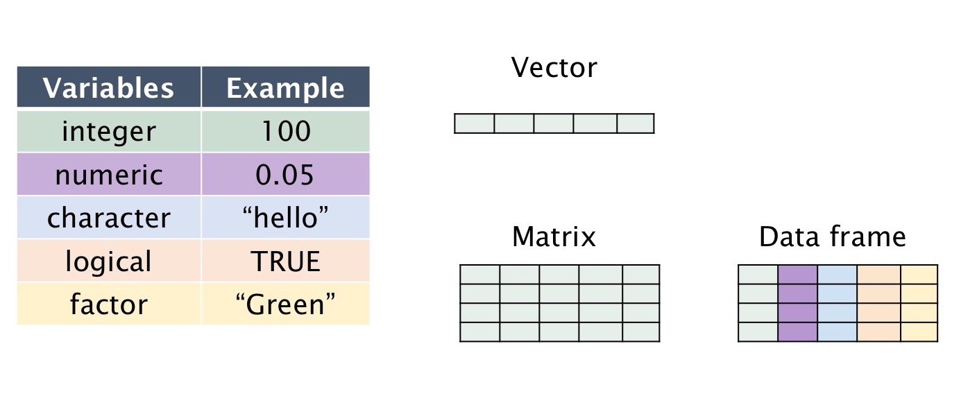
Data Structures in R

Data structures are fundamental components in computer science and programming. They are used to organize, store, and manipulate data efficiently. The choice of the right data structure depends on the specific problem you are trying to solve and the operations you need to perform on the data. Here's an overview of some common data structures used in R -

Scalar

A scalar value refers to a single existing value, it could be in any data form (numeric, character, factor, logical, etc). For example, 1 is a scalar numeric value, 'a' is a scalar character value, F is a scalar logical value.

scalar_numeric <- 1
                        scalar_character <- "a"
                        scalar_logical <- F

Vector

A vector is the most basic data structure in R. It can hold elements of the same data type. Vectors can be numeric, character, logical, or other data types.

numeric_vector <- c(1.2, 2.5, 3.7)
                        character_vector <- c("apple", "banana", "cherry")

Matrices

A matrix is a two-dimensional rectangular data set that contains elements of the same data type arranged in rows and columns. It can be created using a vector input to the matrix() function.

matrix(1:6, nrow = 2, ncol = 3)

Data.frame

A data frame is a two-dimensional data structure where each column can have a different data type. Data frames are commonly used for representing datasets. It can be created using the data.frame() function.

df <- data.frame(Name = c("Alice", "Bob", "Charlie"),
                       \t \t \t Age = c(25, 30, 22))

List

A list is a collection of objects that can be of different data types. It can be created using the list() function.

list(number_vector = 1:3,
                    \t character_vector = c("a", "b", "c"),
                    \t matrix_mine = matrix(1:6, nrow = 2, ncol = 3))

Tables

A table is a special type of data frame used for representing categorical data. It can be created using the table() function.

table(c("a", "b", "c", "a", "b", "c"))

Arrays

An array is a multi-dimensional data structure that can hold elements of the same data type. It can be created using the array() function.

array(1:6, dim = c(2, 3))

Goals of Data Management in R

Data management is the process of ingesting, storing, organizing, and maintaining the data created and collected by an organization. It is a crucial part of the data science workflow. The goals of data management are -

data quality

Data quality refers to the accuracy, completeness, and consistency of data. It is important to ensure data quality because it affects the accuracy of the results of data analysis. Data quality can be improved by performing data cleaning operations such as removing duplicate values, handling missing values, and correcting inconsistent values.

Data Organization

Structure data in a clear and understandable manner. This includes organizing data frames, naming conventions, and creating data dictionaries.

Data Documentation

Document data sources, data cleaning processes, and data transformations. Use comments and metadata to describe variables and datasets.

Data Cleaning

Data cleaning is the process of detecting and correcting corrupt or inaccurate records from a dataset. It is a crucial step in data management because it ensures data quality. Data cleaning can be performed using the dplyr package.

Data Transformation

Data transformation is the process of converting data from one format or structure into another format or structure. It is a crucial step in data management because it ensures data quality. Data transformation can be performed using the dplyr package.

Data Reproducibility

Data reproducibility is the process of reproducing the results of a data analysis. It is a crucial step in data management because it ensures data quality. Data reproducibility can be performed using the dplyr package.

Data Exploration

Data exploration is the process of analyzing data to discover patterns, trends, and relationships. It is a crucial step in data management because it ensures data quality. Data exploration can be performed using the dplyr package.

Data Visualization

Data visualization is the process of representing data in the form of charts, graphs, and maps. It is a crucial step in data management because it ensures data quality. Data visualization can be performed using the ggplot2 package.

Data Communication

Data communication is the process of presenting data in a clear and understandable manner. It is a crucial step in data management because it ensures data quality.

Packages of Interest

There are many packages available in R for data management. Here's an overview of some of the most commonly used packages -

tidyverse

tidyverse is a collection of packages for data management. It provides a set of functions for data manipulation, data visualization, and data communication. It is a part of the tidyverse collection of packages.

install.packages("tidyverse")

The packages available within tidyverse are as follows

dplyr & ggplot2 & tidyr & readr & purrr & tibble & stringr & forcats

Alternatively you can install many of the common packages manually, as below -

Purr

Purr is a package for list manipulation.

install.packages("purr")

dplyr

dplyr is a package for data manipulation. It provides a set of functions for manipulating data frames. It is a part of the tidyverse collection of packages.

install.packages("dplyr")

tidyr

tidyr is a package for data manipulation. It provides a set of functions for manipulating data frames. It is a part of the tidyverse collection of packages.

install.packages("tidyr")

stringr

stringr is a package for string manipulation. It provides a set of functions for manipulating strings. It is a part of the tidyverse collection of packages.

install.packages("stringr")

lubridate

lubridate is a package for date manipulation. It provides a set of functions for manipulating dates. It is a part of the tidyverse collection of packages.

install.packages("lubridate")

readr

readr is a package for data importation. It provides a set of functions for importing data. It is a part of the tidyverse collection of packages.

install.packages("readr")

readxl

readxl is a package for data importation. It provides a set of functions for importing data. It is a part of the tidyverse collection of packages.

install.packages("readxl")

haven

haven is a package for data importation. It provides a set of functions for importing data. It is a part of the tidyverse collection of packages.

install.packages("haven")

jsonlite

jsonlite is a package for data importation. It provides a set of functions for importing data. It is a part of the tidyverse collection of packages.

install.packages("jsonlite")

xml2

xml2 is a package for data importation. It provides a set of functions for importing data. It is a part of the tidyverse collection of packages.

install.packages("xml2")

httr

httr is a package for data importation. It provides a set of functions for importing data. It is a part of the tidyverse collection of packages.

install.packages("httr")

rvest

rvest is a package for data importation. It provides a set of functions for importing data. It is a part of the tidyverse collection of packages.

install.packages("rvest")

pdftools

pdftools is a package for data importation. It provides a set of functions for importing data. It is a part of the tidyverse collection of packages.

install.packages("pdftools")

magick

magick is a package for data importation. It provides a set of functions for importing data. It is a part of the tidyverse collection of packages.

install.packages("magick")

ggplot2

ggplot2 is a package for data visualization. It provides a set of functions for creating plots. It is a part of the tidyverse collection of packages.

install.packages("ggplot2")

Importing Data in R

Before we delve into data importation, it is important to understand the differences between absolute and relative paths.

Absolute Path

An absolute path is a path that points to the same location on one file system regardless of the working directory or combined paths. It is a complete path from start of actual filesystem from / directory.

read.csv("C:\Users\Documents\file.txt")

Relative Path

A relative path is a path that points to the same location on one file system relative to the current working directory. It is a path relative to the current working directory.

setwd("C:\Users\Documents") \br read.csv("file.txt")

In this case, we have set the working directory to "C:\Users\Documents" which allows us to specify the relative path without specifying the entire path.

Data can be imported into R from a variety of sources such as CSV files, Excel files, and databases. Here's an overview of some common data import methods in R -

CSV Files

CSV files are text files that store tabular data in plain text format. They are commonly used for storing data in spreadsheets and databases. CSV files can be imported into R using the read.csv() function.

df <- read.csv("data.csv")

Since CSV files may often stored using different separtors. The following arguments may be of use -

df <- read.csv("data.csv", sep = ",", header = TRUE, stringsAsFactors = FALSE)

dat Files

dat files are text files that store tabular data in plain text format. They are commonly used for storing data in spreadsheets and databases. dat files can be imported into R using the read.table() function.

df <- read.table("data.dat")

Text Files

Text files are files that store text in plain text format. They are commonly used for storing data in spreadsheets and databases. Text files can be imported into R using the readLines() function.

df <- readLines("data.txt")

SPSS Files

SPSS files are files that store data in SPSS format. They are commonly used for storing data in spreadsheets and databases. SPSS files can be imported into R using the haven package.

df <- haven::read_sav("data.sav")

Stata Files

Stata files are files that store data in Stata format. They are commonly used for storing data in spreadsheets and databases. Stata files can be imported into R using the haven package.

df <- haven::read_dta("data.dta")

SAS Files

SAS files are files that store data in SAS format. They are commonly used for storing data in spreadsheets and databases. SAS files can be imported into R using the haven package.

df <- haven::read_sas("data.sas")

Excel Files

Excel files are spreadsheet files that store tabular data in binary format. They are commonly used for storing data in spreadsheets and databases. Excel files can be imported into R using the read_excel() function.

df <- read_excel("data.xlsx")

Database

A database is a collection of data stored in a computer system. It is commonly used for storing data in spreadsheets and databases. Databases can be imported into R using the dbConnect() function.

df <- dbConnect("data.db")

An API is a set of functions and procedures that allow the creation of applications that access the features or data of an operating system, application, or other service. It is commonly used for storing data in spreadsheets and databases. APIs can be imported into R using the httr package.

df <- httr::GET("https://api.data.com")

Web Scraping

Web scraping is the process of extracting data from websites. It is commonly used for storing data in spreadsheets and databases. Web scraping can be performed using the rvest package.

df <- rvest::read_html("https://www.data.com")

Text Files

Text files are files that store text in plain text format. They are commonly used for storing data in spreadsheets and databases. Text files can be imported into R using the readLines() function.

df <- readLines("data.txt")

JSON Files

JSON files are files that store data in JSON format. They are commonly used for storing data in spreadsheets and databases. JSON files can be imported into R using the jsonlite package.

df <- jsonlite::fromJSON("data.json")

XML Files

XML files are files that store data in XML format. They are commonly used for storing data in spreadsheets and databases. XML files can be imported into R using the XML package.

df <- XML::xmlParse("data.xml")

PDF Files

PDF files are files that store data in PDF format. They are commonly used for storing data in spreadsheets and databases. PDF files can be imported into R using the pdftools package.

df <- pdftools::pdf_text("data.pdf")

Images

Images are files that store data in image format. They are commonly used for storing data in spreadsheets and databases. Images can be imported into R using the magick package.

df <- magick::image_read("data.png")

Introducing the Piping Operator

The piping operator is a special operator that allows you to chain multiple operations together. It is a crucial part of the tidyverse collection of packages.

The piping operator, written as %>%, has been a longstanding feature of the magrittr package for R. It takes the output of one function and passes it into another function as an argument. This allows us to link a sequence of analysis steps. For example, we can use the piping operator to chain together multiple operations.

c(1,2,4,5,6,7,8) %>% sum() \br # Typical Code \br sum(1,2,3,4,5,6,7,8)

c(1,2,4,5,6,7,8) %>% sum() %>% mean() \br # Typical Code \br mean(sum(c(1,2,4,5,6,7,8)))

c(1,2,4,5,6,7,8) %>% sum() %>% mean() %>% round() \br # Typical Code \br round(mean(sum(c(1,2,4,5,6,7,8))))

To visualize this process, imagine a factory with different machines placed along a conveyor belt. Each machine is a function that performs a stage of our analysis, like filtering or transforming data. The pipe therefore works like a conveyor belt, transporting the output of one machine to another for further processing.

Dataframes vs Tibbles

	Data Frames	Tibbles
Availability	Base R	Tidyverse
Column Name Conversion	Automatic	None
Data Type Coercion	Automatic	None
Row Names	Enabled by default	Disabled by default
Strict Printing	Less strict	Strict
Subsetting	Use of `[[]]` for columns and `[ ]` for rows	Consistent use of `[]` for both columns and rows
Data Type Columns	Not available	Includes a data type column

Data frames and tibbles are both tabular data structures in R, but they have notable differences. Data frames, part of base R, automatically convert column names, can coerce data types, have row names by default, and offer more relaxed printing. Tibbles, associated with the tidyverse, do not alter column names, avoid data type coercion, exclude row names by default, and provide stricter and more informative printing. Moreover, tibbles allow consistent subsetting and include a data type column. The choice between data frames and tibbles depends on one's preference and the context of data analysis, with tibbles often favored for their user-friendliness within modern data analysis workflows.

                        # Creating a data frame
                        df <- data.frame( 
                        \t    name = c("Alice", "Bob", "Charlie"),
                        \t    age = c(25, 30, 35),
                        \t    gender = c("F", "M", "M")
                        )
                        print(df)
                        # Creating a tibble
                        library(tibble)
                        tb <- tibble(
                         \t   name = c("Alice", "Bob", "Charlie"),
                         \t   age = c(25, 30, 35),
                         \t   gender = c("F", "M", "M")
                        )
                        print(tb)

Tibbles vs Tribbles

	Tibbles	Tribbles
Availability	Part of the tidyverse	Introduced through `tribble`
Column Names	Preserved as is	Specified with `~`
Data Type Coercion	Not automatic	Not automatic
Printing	User-friendly, limited display	User-friendly, limited display

                            # Creating a tibble
                            library(tibble)
                            tb <- tibble(
                             \t   name = c("Alice", "Bob", "Charlie"),
                             \t   age = c(25, 30, 35),
                             \t   gender = c("F", "M", "M")
                            )
                            print(tb)
                            
                            # Creating a tribble
                            library(tibble)
                            trb <- tribble(
                                \t  ~name, ~age, ~gender,
                                \t  "Alice", 25, "F",
                                \t  "Bob", 30, "M",
                                \t  "Charlie", 35, "M"
                            )
                            print(trb)

Dplyr Functions

Category	Function	Utility
Data frame verbs (Rows)	arrange()	Order rows using column values
Data frame verbs (Rows)	distinct()	Keep distinct/unique rows
Data frame verbs (Rows)	filter()	Keep rows that match a condition
Data frame verbs (Rows)	slice()	Subset rows using their positions
Columns	mutate()	Create, modify, and delete columns
Columns	select()	Keep or drop columns using their names and types
Groups	group_by()	Group data by one or more variables
Data frames	bind_cols()	Bind multiple data frames by column
Data frames	bind_rows()	Bind multiple data frames by row
Vector functions	between()	Detect where values fall in a specified range
Vector functions	coalesce()	Find the first non-missing element

In simple words, the dplyr package in R is like a set of powerful tools that help you easily and efficiently manipulate and transform data in data frames. It provides functions for filtering, sorting, summarizing, and modifying your data so that you can perform tasks like data cleaning and analysis with less code and more clarity. Think of it as a Swiss Army knife for working with data tables in R.

Arrange Function

The arrange() function is used to sort rows in ascending or descending order. It takes a data frame as input and returns a data frame with the rows sorted in ascending or descending order.

                            # Sort rows in ascending order
                            df <- arrange(df, age)
                            # Sort rows in descending order
                            df <- arrange(df, desc(age))

Distinct Function

The distinct() function is used to remove duplicate rows from a data frame. It takes a data frame as input and returns a data frame with the duplicate rows removed.

                            # Remove duplicate rows
                            df <- distinct(df)

Filter Function

The filter() function is used to select rows that match a condition. It takes a data frame as input and returns a data frame with the rows that match the condition.

                            # Select rows where age is greater than 30
                            df <- filter(df, age > 30)

Filtering with if_any(), if_all(), and between()

Function	Description	Example
if_any()	Filter rows if any of the specified conditions are met.	library(dplyr) # Sample data frame data <- data.frame( Name = c("Alice", "Bob", "Charlie", "David"), Age = c(25, 30, 22, 28), Score = c(90, 75, 85, 95) ) filtered_data <- data %>% filter(if_any(c(Age, Score), ~ . >= 30))
if_all()	Filter rows if all of the specified conditions are met.	library(dplyr) # Sample data frame data <- data.frame( Name = c("Alice", "Bob", "Charlie", "David"), Age = c(25, 30, 22, 28), Score = c(90, 75, 85, 95) ) filtered_data <- data %>% filter(if_all(c(Age, Score), ~ . >= 30))
between()	Filter rows where a variable's value is within a specified range.	library(dplyr) # Sample data frame data <- data.frame( Name = c("Alice", "Bob", "Charlie", "David"), Age = c(25, 30, 22, 28), Score = c(90, 75, 85, 95) ) filtered_data <- data %>% filter(between(Age, 25, 30))

Function

Description

Example

if_any()

Filter rows if any of the specified conditions are met.

            library(dplyr)

            # Sample data frame
            data <- data.frame(
            Name = c("Alice", "Bob", "Charlie", "David"),
            Age = c(25, 30, 22, 28),
            Score = c(90, 75, 85, 95)
            )

            filtered_data <- data %>%
            filter(if_any(c(Age, Score), ~ . >= 30))

if_all()

Filter rows if all of the specified conditions are met.

            library(dplyr)

            # Sample data frame
            data <- data.frame(
            Name = c("Alice", "Bob", "Charlie", "David"),
            Age = c(25, 30, 22, 28),
            Score = c(90, 75, 85, 95)
            )

            filtered_data <- data %>%
            filter(if_all(c(Age, Score), ~ . >= 30))

between()

Filter rows where a variable's value is within a specified range.

            library(dplyr)

            # Sample data frame
            data <- data.frame(
            Name = c("Alice", "Bob", "Charlie", "David"),
            Age = c(25, 30, 22, 28),
            Score = c(90, 75, 85, 95)
            )

            filtered_data <- data %>%
            filter(between(Age, 25, 30))

Mutate Function

The mutate() function is used to create new columns or modify existing columns. It takes a data frame as input and returns a data frame with the new or modified columns.

                        # Create a new column
                        df <- mutate(df, age_group = ifelse(age < 30, "young", "old"))
                        # Modify an existing column
                        df <- mutate(df, age = age + 1)

Using mutate() with across() and c_across()

Function	Description	Example
across()	Apply a function or functions to multiple columns simultaneously within the mutate() function.	library(dplyr) # Sample data frame data <- data.frame( Name = c("Alice", "Bob", "Charlie", "David"), Math_Score = c(90, 75, 85, 95), English_Score = c(88, 92, 78, 86) ) mutated_data <- data %>% mutate(across(.cols = starts_with("Math"), .fns = ~ . * 1.1))
c_across()	Combine values from multiple columns into a single column within the mutate() function.	library(dplyr) # Sample data frame data <- data.frame( Name = c("Alice", "Bob", "Charlie", "David"), Math_Score = c(90, 75, 85, 95), English_Score = c(88, 92, 78, 86) ) mutated_data <- data %>% mutate(Total_Score = c_across(starts_with("Score")))

Function

Description

Example

across()

Apply a function or functions to multiple columns simultaneously within the mutate() function.

        library(dplyr)

        # Sample data frame
        data <- data.frame(
        Name = c("Alice", "Bob", "Charlie", "David"),
        Math_Score = c(90, 75, 85, 95),
        English_Score = c(88, 92, 78, 86)
        )

        mutated_data <- data %>%
        mutate(across(.cols = starts_with("Math"), .fns = ~ . * 1.1))

c_across()

Combine values from multiple columns into a single column within the mutate() function.

        library(dplyr)

        # Sample data frame
        data <- data.frame(
        Name = c("Alice", "Bob", "Charlie", "David"),
        Math_Score = c(90, 75, 85, 95),
        English_Score = c(88, 92, 78, 86)
        )

        mutated_data <- data %>%
        mutate(Total_Score = c_across(starts_with("Score")))

Select Function

The select() function is used to select columns from a data frame. It takes a data frame as input and returns a data frame with the selected columns.

                        # Select columns by name
                        df <- select(df, name, age)
                        # Select columns by type
                        df <- select(df, where(is.numeric))
                        # Select columns by position
                        df <- select(df, 1:3)

Selecting with starts_with(), ends_with(), contains(), and matches()

Function	Description	Syntax
starts_with()	Select columns that start with a specific prefix.	`select(starts_with("prefix"))`
ends_with()	Select columns that end with a specific suffix.	`select(ends_with("suffix"))`
contains()	Select columns that contain a specific substring.	`select(contains("substring"))`
matches()	Select columns based on regular expressions.	`select(matches("regex_pattern"))`
everything()	Select all columns.	`select(everything())`
where()	Select columns based on a predicate function.	`select(where(is.numeric))`

Group By and Summarise Function

The group_by() function is used to group rows by one or more variables. It takes a data frame as input and returns a data frame with the rows grouped by the specified variables.

The summarise() function is used to summarise data by collapsing multiple values into a single value. It is often used in conjunction with the group_by() function to summarise data by groups.

                library(dplyr)

                # Sample data frame
                data <- data.frame(
                Name = c("Alice", "Bob", "Charlie", "David"),
                Math_Score = c(90, 75, 85, 95),
                English_Score = c(88, 92, 78, 86)
                )

                grouped_data <- data %>%
                group_by(Name) %>%
                summarise(Average_Math_Score = mean(Math_Score), Average_English_Score = mean(English_Score))

Vector Functions in dplyr

Function	Description
between()	Detect where values fall in a specified range.
case_match()	A general vectorized switch() function.
case_when()	A general vectorized if-else function.
coalesce()	Find the first non-missing element among multiple vectors.
consecutive_id()	Generate a unique identifier for consecutive combinations of values.
cumall(), cumany(), cummean()	Cumulative versions of any(), all(), and mean() functions.
desc()	Sort data in descending order.
if_else()	Vectorized if-else function.
lag(), lead()	Compute lagged or leading values in a vector.
n_distinct()	Count unique combinations in a vector.
na_if()	Convert specified values to NA in a vector.
near()	Compare two numeric vectors to check if they are nearly equal.
nth(), first(), last()	Extract the nth, first, or last value from a vector.
ntile()	Bucket a numeric vector into n groups based on quantiles.
order_by()	A helper function for ordering in window functions.
percent_rank(), cume_dist()	Proportional ranking functions for a vector.
recode(), recode_factor()	Recode values in a vector.
row_number(), min_rank(), dense_rank()	Integer ranking functions for a vector.

Using case_when() and case_match()

# Example for case_match()
            library(dplyr)

            data <- data.frame(Category = c("A", "B", "C", "D"))

            mutated_data <- data %>%
            mutate(Result = case_match(Category, "A" = "Alpha", "B" = "Beta", "C" = "Charlie"))

# Example for case_when()
            library(dplyr)

            data <- data.frame(Score = c(80, 95, 60, 75))

            mutated_data <- data %>%
            mutate(Grade = case_when(
                Score >= 90 ~ "A",
                Score >= 80 ~ "B",
                Score >= 70 ~ "C",
                TRUE ~ "D"
            ))

Using if_else() with mutate()

                library(dplyr)

                data <- data.frame(Score = c(80, 95, 60, 75))

                mutated_data <- data %>%
                mutate(Grade = if_else(Score >= 90, "A", "B"))

Using lag() and lead() with mutate()

                library(dplyr)

                data <- data.frame(Score = c(80, 95, 60, 75))

                mutated_data <- data %>%
                mutate(Lagged_Score = lag(Score), Leading_Score = lead(Score))

Joining Datasets

Function	Description
anti_join()	Return rows from the left table that are not present in the right table.
full_join()	Return all rows from both tables.
inner_join()	Return rows that match in both tables.
left_join()	Return all rows from the left table.
right_join()	Return all rows from the right table.
semi_join()	Return rows from the left table that are present in the right table.

ID	Name
1	Alice
2	Bob
3	Charlie
4	David

ID	Score
2	95
3	89
5	78
6	92

Using Join Functions

                library(dplyr)

                # Sample data frames
                left_data <- data.frame(
                Name = c("Alice", "Bob", "Charlie", "David"),
                Age = c(25, 30, 22, 28)
                )

                right_data <- data.frame(
                Name = c("Alice", "Bob", "Charlie", "David"),
                Score = c(90, 75, 85, 95)
                )

                # Join data frames
                joined_data <- left_data %>%
                inner_join(right_data, by = "Name")

Tranform Datasets

The gather() function is used to transform a dataset from wide format to long format. It takes a data frame as input and returns a data frame with the columns gathered into key-value pairs.

                library(tidyr)

                # Sample data frame
                data <- data.frame(
                Name = c("Alice", "Bob", "Charlie", "David"),
                Math_Score = c(90, 75, 85, 95),
                English_Score = c(88, 92, 78, 86)
                )

                # Gather columns
                gathered_data <- data %>%
                gather(key = "Subject", value = "Score", Math_Score, English_Score)

Spread Datasets

The spread() function is used to transform a dataset from long format to wide format. It takes a data frame as input and returns a data frame with the key-value pairs spread across multiple columns.

                library(tidyr)

                # Sample data frame
                data <- data.frame(
                Name = c("Alice", "Bob", "Charlie", "David"),
                Math_Score = c(90, 75, 85, 95),
                English_Score = c(88, 92, 78, 86)
                )

                # Spread columns
                spread_data <- data %>%
                gather(key = "Subject", value = "Score", Math_Score, English_Score)

Separate Datasets

The separate() function is used to separate a column into multiple columns. It takes a data frame as input and returns a data frame with the column separated into multiple columns.

                library(tidyr)

                # Sample data frame
                data <- data.frame(
                Name = c("Alice", "Bob", "Charlie", "David"),
                Age = c("25, 30", "30, 35", "22, 27", "28, 33")
                )

                # Separate column
                separated_data <- data %>%
                separate(Age, into = c("Age_1", "Age_2"), sep = ", ")

Unite Datasets

The unite() function is used to unite multiple columns into a single column. It takes a data frame as input and returns a data frame with the columns united into a single column.

                library(tidyr)

                # Sample data frame
                data <- data.frame(
                Name = c("Alice", "Bob", "Charlie", "David"),
                Age_1 = c(25, 30, 22, 28),
                Age_2 = c(30, 35, 27, 33)
                )

                # Unite columns
                united_data <- data %>%
                unite(Age, Age_1, Age_2, sep = ", ")

Name	Exam 1	Exam 2	Exam 3
Spread Data (Wide Form)
Alice	85	88	78
Bob	90	92	85
Charlie	78	86	92

Name	Exam	Score
Gathered Data (Long Form)
Alice	Exam_1	85
Bob	Exam_1	90
Charlie	Exam_1	78
Alice	Exam_2	88
Bob	Exam_2	92
Charlie	Exam_2	86
Alice	Exam_3	78
Bob	Exam_3	85
Charlie	Exam_3	92

Brief Introduction to R Markdown

R Markdown is a file format for making dynamic documents with R. An R Markdown document is written in markdown (an easy-to-write plain text format) and contains chunks of embedded R code. R Markdown files are designed to be used with the rmarkdown package. R Markdown files have the file extension “.Rmd”. When you render an R Markdown document, R Markdown converts your document into the desired output format.

Setting up a R Markdown file -

When you open a new R Markdown file in RStudio, a pop-up window appears that prompts you to select output format to use for the document. You can select from a variety of output formats including HTML, PDF, MS Word, and more. You can also select the default output format for all new R Markdown files in the R Markdown preferences.

R Markdown Syntax

R Markdown files are written using markdown, a lightweight markup language that is easy to read and write. Markdown is a way to style text on the web. You control the display of the document; formatting words as bold or italic, adding images, and creating lists are just a few of the things we can do with Markdown. Mostly, Markdown is just regular text with a few non-alphabetic characters thrown in, like # or *.

R Markdown Syntax	Description
`# Header 1`	Create a top-level heading (Header 1).
`## Header 2`	Create a second-level heading (Header 2).
`Italic`	Italicize text using asterisks.
`Bold`	Make text bold using double asterisks.
`[Link](https://example.com)`	Create a hyperlink with the specified text and URL.
`![Image](image.png)`	Embed an image in the document with alt text and image source.
`> Blockquote`	Create a blockquote for cited content.
`* List item 1`	Add an unordered list item with an asterisk.
`1. Numbered item`	Include a numbered list item.
`---`	Insert a horizontal rule (horizontal line).
`Inline code syntax`	Mark inline code using backticks.
``` `Code block` ```	Create a code block for displaying and formatting code.

Embedding R Code in R Markdown

R Markdown files can contain chunks of embedded R code. You can embed an R code chunk in an R Markdown file by using the chunk option in the RStudio toolbar. You can also use the keyboard shortcut Ctrl + Alt + I (Windows/Linux) or Cmd + Option + I (Mac).

Option	Value	Description
eval	TRUE	Whether to evaluate the code and include its results
echo	TRUE	Whether to display code along with its results
warning	TRUE	Whether to display warnings
error	FALSE	Whether to display errors
message	TRUE	Whether to display messages
tidy	FALSE	Whether to reformat code in a tidy way when displaying it
results	"markup"	Output format for code results (e.g., "markup", "asis", "hold", or "hide")
cache	FALSE	Whether to cache results for future renders
comment	"##"	Comment character to preface results with
fig.width	7	Width in inches for plots created in the chunk
fig.height	7	Height in inches for plots created in the chunk

About Me

I am a 2nd year PhD student in the Quanitative Methods Department at York University. Although my research primary revolves around adapting machine learning methodologies to Psychology, I take immense pleasure in improving the statistical literacy for everyone involved.

My research interests include = Machine Learning, Psychometrics, statistical pedagogy, and Data Science.

My hobbies include = Jiu Jitsu, Coding, Working Out, and Reading.

“Success is not final, failure is not fatal: It is the courage to continue that counts.” - Winston S. Churchill